Learning tmap: Dipping my toes in the R-spatial world

I’ve been wanting to wade into the R spatial waters for some time, and now I’ve finally gotten around to it!

In case you didn’t know, R has a whole community built around spatial data viz and data science.

I made a few maps previously with ggplot2, but as a raging perfectionist, I was left longing for more control. The nagging need to map with something else was kickstarted when I discovered that plotly and chloropleth maps don’t always get along. And that’s how I ended up dabbling with tmap.

Fortunately, tmap prides itself on being like a ggplot2 built specifically for mapping – and high visual quality ones at that. When you need an interactive map, leaflet joins the party.

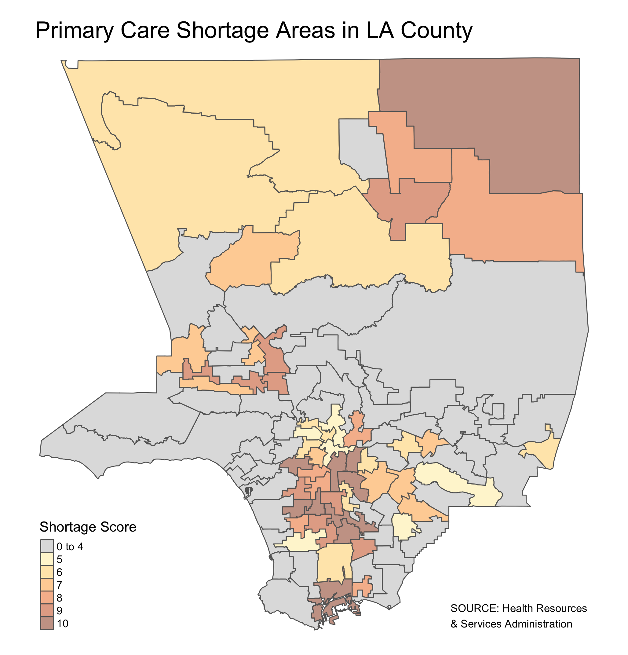
In the examples below, I took California’s 2020 data on Primary Care Shortage Areas and visualized Los Angeles County by state-designated Medical Service Study Areas. (Note: I had to alter the geoJSON for one of the MSSAs to get rid of Catalina Island and San Clemente Island, which were messing up the overall map size.)

Code

library(sf)
library(tidyverse)
library(tmap)
library(tmaptools)
library(leaflet)

laco <- read_sf("data/lacoG.geojson")

labelItems <- sprintf(
  "<strong>Area: </strong>%s<br/><strong>Shortage Score: </strong>%s<br/><strong>Population: </strong>%s<br/><strong>Pop. Under Poverty Line: </strong>%s<br/><strong>Provider-to-Civilian Ratio: </strong>%s<br/>",laco$MSSA_NAME, laco$PCSA_SCORE, laco$POP, laco$POV_RATE, laco$PC_PHYS_R_CIV
) %>% lapply(htmltools::HTML)

laco <- laco %>%
  mutate(labelText = labelItems)

lacoSta <- tm_shape(laco) +
  tm_polygons(col = "PCSA_SCORE",
              id = "MSSA_NAME",
              title = "Shortage Score",
              breaks = c(0, 5, 6, 7, 8, 9, 10, 11), 
              labels = c("0 to 4", "5", "6", "7", "8", "9","10"),
              palette = c("0 to 4" = "gray75",
                          "5" = "#feeca5",
                          "6" = "#fecf66",
                          "7" = "#fea332",
                          "8" = "#ec7114",
                          "9" = "#c74a02",
                          "10" = "#8e3003"),
              alpha = 0.5) +
  tm_credits("SOURCE: Health Resources\n& Services Administration", position = c("right", "bottom")) +
  tm_layout(
    main.title = "Primary Care Shortage Areas in LA County",
    frame = FALSE
  )

tmap_save(tm = lacoSta, 
          filename = "images/lacoSta.png")

Remember when I said it works kind of like ggplot2? You can see what I mean when it comes to how things are layered. First you see the tm_polygons call. The layers use some kind of tm_xxxxx() call akin to geom_xxxxx(). Next layer is tm_credits() similarly to how you might use labs() for plots. And think of tm_layout() offering that detailed customization that you get from theme() for plots.

Making the interactive version took a long dig into the documentation to get things exactly how I wanted them finally, but I was more than happy with the finished product. It’s also nice that you don’t necessarily even have to make two wholly different maps. If you’re not picky about some of the interactive map’s details, you can use the tmm() command to flip back and forth between static and interactive views of the same map.

Code

lacoInt <- tm_shape(laco) +
  tm_basemap(server = "OpenStreetMap") +
  tm_polygons(col = "PCSA_SCORE",
              id = "MSSA_NAME",
              title = "Shortage Score",
              breaks = c(0, 5, 6, 7, 8, 9, 10, 11), 
              labels = c("0 to 4", "5", "6", "7", "8", "9","10"),
              palette = c("0 to 4" = "gray75",
                          "5" = "#feeca5",
                          "6" = "#fecf66",
                          "7" = "#fea332",
                          "8" = "#ec7114",
                          "9" = "#c74a02",
                          "10" = "#8e3003"),
              alpha = 0.6,
              popup.vars = c("Shortage Score" = "PCSA_SCORE", 
                             "Population" = "POP", 
                             "Poverty Rate" = "POV_RATE", 
                             "Provider-to-Civilian Ratio" = "PC_PHYS_R_CIV")) +
  tmap_options(
    output.size = 1600
  ) 

tmap_mode("view")
htmltools::h3("Primary Care Shortage Areas in LA County")

Primary Care Shortage Areas in LA County

Code

lacoInt

If this whet your appetite to start toying with tmap, here are some helpful starting points:

tmap Github

r-spatial.org

Geocomputation with R

tmap: Elegant and Effective Informative Maps book (incomplete)

Did I miss a good one? Comment and shout it out!